Kingdom Knapsack
Here’s what happens when you bring your day job to church.
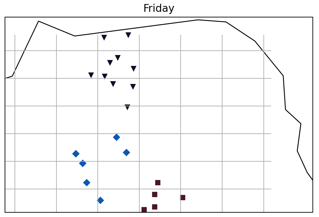
An example of the groups created from sample data. Can you tell the black line is supposed to be the outline of San Francisco?
We as communal creatures do life best with other people by our side, and Christians are no exception. In Acts 5 at the inception of the Christian church, we see the apostles flogged and ordered to stop talking about Jesus, yet
Day after day, in the temple courts and from house to house, they never stopped teaching and proclaiming the good news that Jesus is the Messiah.
The “house to house” phrase is the inspiration for the name of my software, Oikoi, which is Greek for “houses”. And yes, a singular “house” is the yogurt brand you’re thinking of. Many churches, mine included, facilitate house meetings throughout the week for the corporate reading of Scripture, life sharing, and communal prayer. Being a large church in San Francisco, however, brings about a couple factors key to why there was a need for some keyboard slapping:
- People move constantly. Rebalancing these groups in light of geography is a must.
- People are busy. In a rise-and-grind city, many folks have strong restrictions on their availability.
Our church has a consistent need to spin up new small groups when congregants find bandwidth to join, move across town and want to find hyperlocal community, or join the church for the first time. Previously, three times a year, a small group of people drags names around spreadsheets to try to find a reasonable grouping of ~100 people, balancing for location and with a preference towards diversity of life stage. All things equal, an age and life stage disparity brings a certain kind of richness, and in fact a large reason I stuck with my group when I moved to the city was the wide array of backgrounds, cultures, ages, and occupations in our living room as we all pursued the same thing.
I’ve been learning a lot of ML techniques during my job search, so I was super eager to tackle this problem with some fancy gradient descent or simulated annealing. The issue I ran into is the following constraints on groups:
- Groups have a minimum and maximum size (8-12 people)
- Groups can only meet on days when all members are available
The goal of most optimization problems is to find the lowest cost of a system, and this is no different - the “cost” of a small group would be the distance its members have to travel. I was hoping to teach the computer how to hike down a mountain range: a continuous cost function where each step took you to lower elevation. Instead, imagine a trail on a piece of Swiss cheese while blindfolded - there’s no way to tell if any other direction will lead to lower elevation, and a lot of the time, there’s a giant hole where you want to step. A large number of possibilities exist where the groups violate the constraints above, so I couldn’t do a lot of fancy trail-walking. Instead, the problem is more like landing a helicopter at a random point on this cheese and hoping it’s not in a hole.
Take 1: “Rapid”-fire helicopter landing

To give an idea of how big this sample space is, consider that each person has to decide which day they’re attending small group. For the sake of example, let’s say that busy San Franciscans can only meet on average 2.5 days a week. That still means that for p participants, there are about \((2.5)^p\) options. For \(p = 100\), that’s 6 duodecillion (that’s 39 zeros). Yike. But isn’t that where machines come in? Yeah, there are a lot of helicopters to land, but software can land helicopters really really fast, right?
That’s what I assumed when I drafted this first algorithm. After landing a helicopter, i.e. deciding for each person what day they were attending, the optimal group was determinable. We’re minimizing the distance each person is from the center of the group:
\[L = \sum_{i=0}^{n} \sqrt{(x_i - \bar{x})^2 + (y_i - \bar{y})^2}\]The tricky part is, of course, that the center of the group is determined by the people in the group, so the cost changes depending on the group composition. So I thought it was a good idea to step through all possible compositions of the groups for a given day.
For \(p_d\) participants on a given day, you could have as few as \(\left\lfloor \frac{p_d}{12} \right\rfloor\) groups or as many as \(\left\lfloor \frac{p_d}{8} \right\rfloor\), since the groups are of 8 to 12 people. Let’s call the number of groups g. For each valid number of groups g, we consider the partitions of \(p_d\) of length g where each number is a valid group size. A partition is just a potential sum, e.g. 4+5 and 1+1+6+1 are valid partitions of 9, and 8+8+8 and 12+12 are valid partitions of 24. These partitions represent the different ways group sizes could be formed: one group of 8 and one group of 10 might be less costly than two groups of 9.
Once we have the different group sizings, we test each way of packing all the participants into each group. How many ways are there to pick participants for these group sizes? Where \(g_i\) for \(1 \le i \le |g|\) is a given group, we have:
\[\left( \frac{p}{|g_1|} \right) \times \left( \frac{p - |g_1|}{|g_2|} \right) \times \cdots = \prod_{i=0}^{|g|-1} \left( \frac{p - |g_i|}{|g_{i+1}|} \right)\]We iterate through all but the last group because the last group decision is moot - it’s just whoever is left.
As fun as it was to figure all this out, this giant product is part of why it took like an hour to land a single helicopter. Back to the drawing board.
Take 2: Mathy cartography

The next idea seemed a little more computationally tenable. The computer is now a cartographer, creating seven maps of the Bay Area, one for each day of the week. Each participant gets a point on the map of each day they’re available. Once the maps are drawn up, it picks a map to read, finds an appropriately sized group of points on that map, and places the corresponding people into a group, removing the group’s other points on other maps. The cartographer keeps picking groups of points from different maps until it gets tired, and then it examines any remaining points and tries to throw those people into groups it has already created.
To find a cluster of points that are close enough to each other, I chose the Density-Based Spatial Clustering of Applications with Noise (DBSCAN) algorithm. This algorithm defines two parameters: epsilon (ε), the maximum distance between two points for them to be considered as neighbors, and min_pts, the minimum number of neighbors required for a point to be considered a core point. This algorithm loops through all the points and categorizes each as either a core point (a point with min_pts - 1 neighbors), border point (neighbors of core points that aren’t core points), or noise point (the rest). The noise is ignored, and a cluster consists of any neighbor core point(s) and their border points. Empirically, I got convergence with sample data for min_pts=8, so the groups always had just one core point.
When the carto-computer spends a long time trying to find clusters for a given ε to no avail, ε is increased so it can continue looking for candidate clusters. This happens until the number of people left can’t make a new cluster, or we’ve tried increasing ε enough times without any new clusters.
While there’s slight variation depending on how ε grows and different sample data, it now takes a couple of seconds to look at all the maps and either make a set of groups or get tired and give up. Our runs with actual data involve ~10,000 cartography sessions, recommending the lowest-cost group arrangement across all of the sessions.
As a result, we placed 66 new people into 7 different community groups this month! Happy to have written something useful for many future iterations, and it’s great to have a hand in connecting people in San Francisco.